Using the GUI

Once you’ve run the processing, you can open the output stat.npy file from the GUI. This allows you to explore the data in depth both spatially and in time. In addition you can classify ROIs as ‘cells’ or ‘NOT cells’ (left or right side of screen) and train a classifier to automatically identify the cells as one of these two classes. Note that these categories do not have to be ‘cells’ and ‘NOT cells’, they could be ‘boutons’ and ‘NOT boutons’, we just chose to say ‘cells’ because that’s the most common ROI studied.

You can now drag and drop your stat.npy files into the GUI!

Different views and colors for ROI panels

Views

To turn off ROIs in views 2-4, uncheck ROIs on

1. ROIs: ROIs only are drawn

2. mean img: mean image is shown in background

3. mean img (enhanced): mean image filtered with a min-max filter shown in background

4. correlation map: map of correlated pixels shown in background

5. mean img (non-functional): the non-functional mean image shown in background (if nchannels=2)

Colors

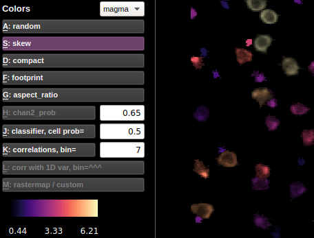
Randomly colored ROI view is the default view. The ROIs in the random view are colored between purple and yellow, with red reserved for ROIs assigned to be RED based on the non-functional channel (you can change the threshold for calling a cell RED with the number next to the chan2 prob button). The other color views color the ROIs based on their statistics. The values of those statistics are shown in the colorbar below the buttons.

Here is more info about the less explanatory views:

Correlations

In correlation color view, the selected cell’s activity (or the mean of the selected cells’ activities) is correlated with the activity of all the other ROIs. The ROIs are colored according to these correlations. The bin in which to compute the correlations can be chosen (in units of frames). The default bin size is the number of frames per second (ops['fs']).

If a 1D external variable is loaded, then the corr with 1D var button is activated. The cells are then colored according to their correlation with the external variable. The bin size is determined by the box next to the correlations button.

Correlations with 1D var

You can load an external stimulus or behavioral trace (1D) using “File - Load behavior or stim trace (1D only)”. The GUI expects a *.npy file that is the same length as the data in time (F.shape[1] from “F.npy”). You can then look at the correlation of each cell with this trace. And it will be plotted along with the cell traces if you select multiple cells or in the “Visualize” menu.

Rastermap / custom

Rastermap: Click ‘Visualize selected cells’ in the Visualizations menu and run rastermap on the cells. The selected cells (which could be all cells on LEFT or RIGHT) will then be colored based on their position in the rastermap.

Custom map: Use ‘Load custom hue’ in the Visualizations menu to load a *.npy file with the same number of values as ROIs (length of stat) and these values will become the hues of the cells (scaled to between 0 and 1) for the HSV map. If you do rastermap after this then the colors will change and vice versa this will overwrite the rastermap colors.

Buttons / shortcuts for cell selection

Mouse control

• double left click = returns to full view in ALL PLOTS

• left click = select cell

• left click + CTRL = select multiple cells

• left click + drag = moves field of view

• right click = flip selected cell(s) from left<->right, – or if clicked in trace view, will open up “export” option

• scroll wheel = zoom in and out

Keyboard shortcuts

• Esc = returns to full view

• Delete = removes box from draw selection from window For the letters, just press the letter (do not capitalize)

• O = turn of ROIs in non-ROI view

• Q-U = different views (can change saturation with slider)

• A-M = different color maps

• Left and right keys = cycle between cells of same panel

• Up Key = flip selected cell to other panel

• Alt+Enter = merge selected ROIs

• note you can also ask the GUI to auto-suggest merges with the Merge>Auto-suggest merges window *

Multi-cell selection

You can select multiple cells by holding down CTRL while left-clicking on cells. If you are in ‘cells’ or ‘NOT cells’ view (not ‘both’ view), then several buttons for multi-cell selection activate.

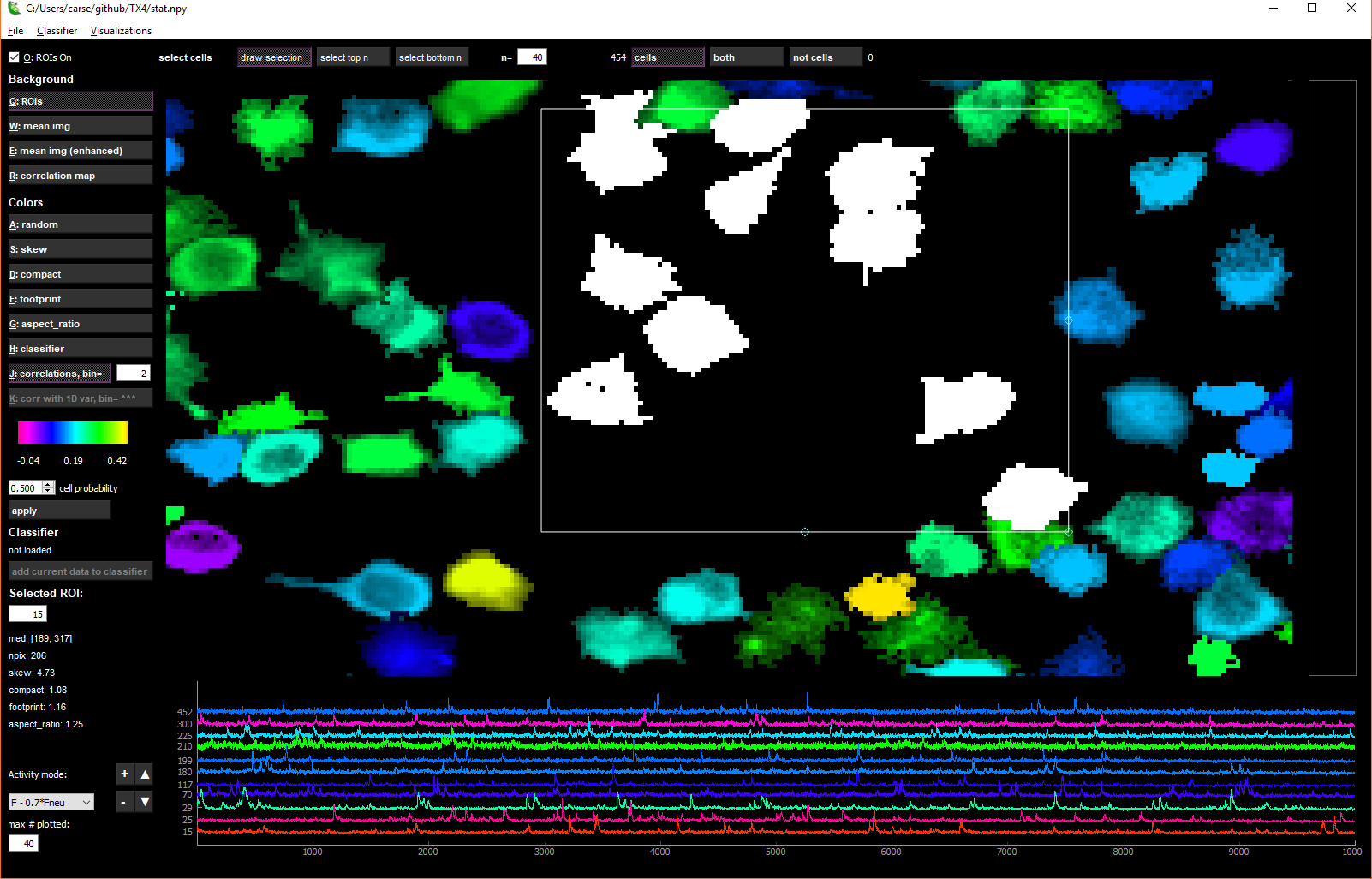
The draw selection button activates a box that you can drag and resize to select multiple cells. To delete the box, click the Delete key. select top n selects n=X top neurons from the current colormap. For instance, in ‘skew’ view, select top n will select the most skewed neurons. In ‘correlation’ view, it will choose the most correlated neurons with the currently selected neuron.

Trace view (bottom row)

When one cell is selected, the fluorescence, neuropil and deconvolved traces are shown for the chosen cell in the bottom row of the GUI. When multiple cells are selected, you can choose what type of traces to view with the drop-down menu in the lower left:

• F: fluorescence

• Fneu: neuropil fluorescence

• F - 0.7*Fneu: corrected fluorescence

• deconvolved: deconvolution of corrected fluorescence

You can resize the trace view with the triangle buttons (bigger = ▲, smaller = ▼). If multiple cells are selected, you can vary how much the traces overlap with the +/- buttons.

You can select as many cells as you want, but by default only 40 of those will be plotted. You can increase or decrease this number by changing the number in the box below max # plotted.

You can hide the fluorescence, neuropil and/or the deconvolved traces by toggling the chechboxes or using the keys as follows:

Deconvolved - N key Neuropil - B Key Fluorescence - V Key

Classifying cells

suite2p comes with a built-in classifier (based on our own manual curation of GCaMP6s imaging of cells in cortex). The default classifier is initialized as the built-in classifier, but can be modified by the user.

After running suite2p, the cells are automatically classified by the default classifier (at the time of running the pipeline), and these cell probabilities are shown as the colors in the classifier view. You can then further manually curate this data (flipping cells left and right depending on your criteria).

Adding data to a classifier

You can add this manually curated data to an already built classifier:

1. Load a classifier by going to the “Classifier” menu and clicking “Load”. Choose the default classifier, or load another classifier that you’ve built and saved with the from file option.

2. Click the add current data to classifier button. This will either overwrite the classifier file that is loaded, or you can specify a file location for the classifier with this newly added data.

Building your own classifier

Go to the “Classifier” menu and click “Build”. A window will pop up and in the window you can add datasets as training samples for the classifier. Click the Load iscell.npy button and add an iscell.npy file. You can add as many as you like, then click build classifier, and it will ask you to specify a file location for the new classifier. Then you can load the classifier that you built into the GUI, or you can save it as your default classifier.

Visualizing activity

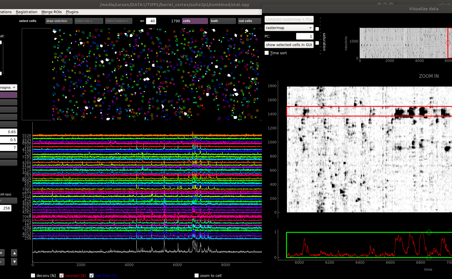
Go to the “Visualizations” menu and click “Visualize selected cells”. If only one ROI is selected, then all ROIs in that view (cell or not cell) will be plotted. Otherwise the selected cells are plotted. You can sort the neurons by their principal component weights, or by our algorithm rastermap by clicking the compute buttons. Once you click the compute buttons, they will be grayed out, because you can’t compute them again (they won’t change). The plot below shows a mesoscope recording sorted by rastermap. You can change between sorting by rastermap and by the PCs by using the drop-down menu.

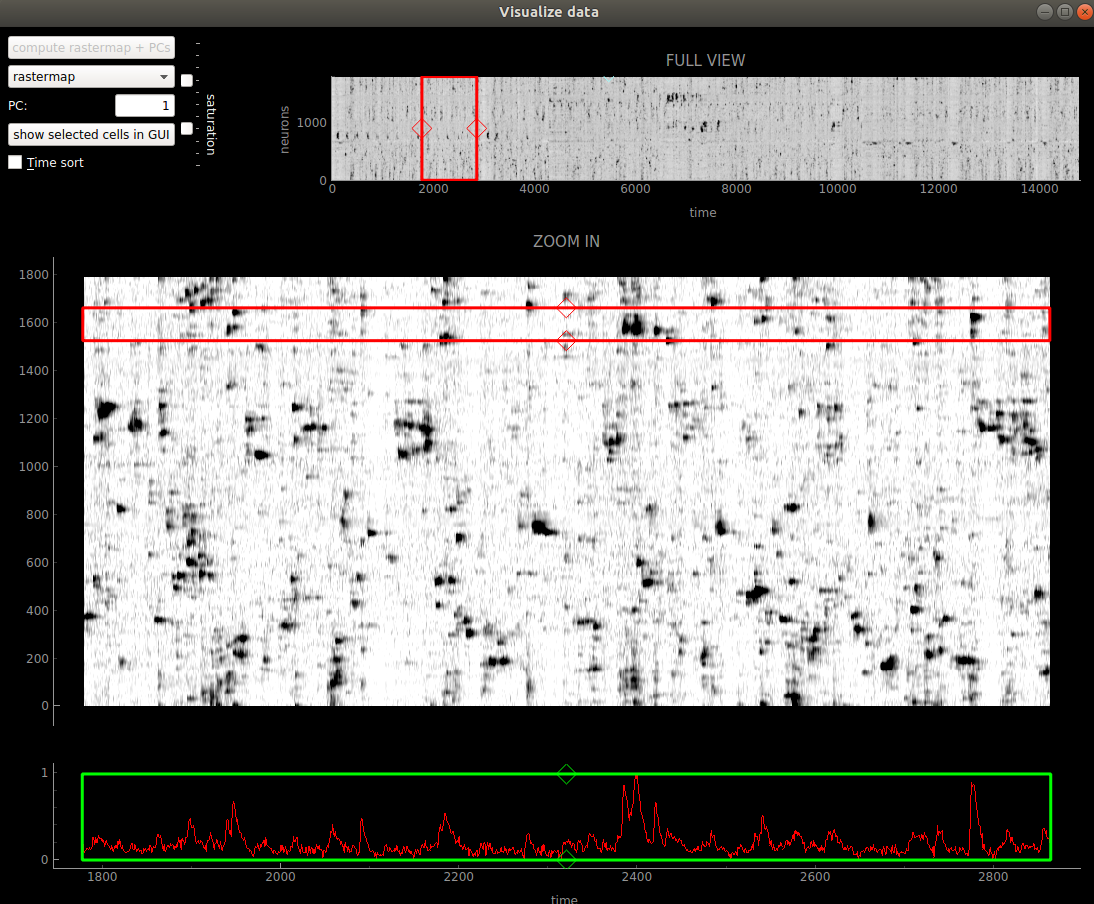
The red box allows you to zoom in on specific segments of the recording. You can move it by dragging the mouse when in the box, or with the arrow keys. You can resize it by using the diamond handles on the sides of the box, or by holding down the shift key and using the arrow keys.

If you click the show selected cells in GUI button, then the cells surrounded by the red box will show up as white in the GUI.

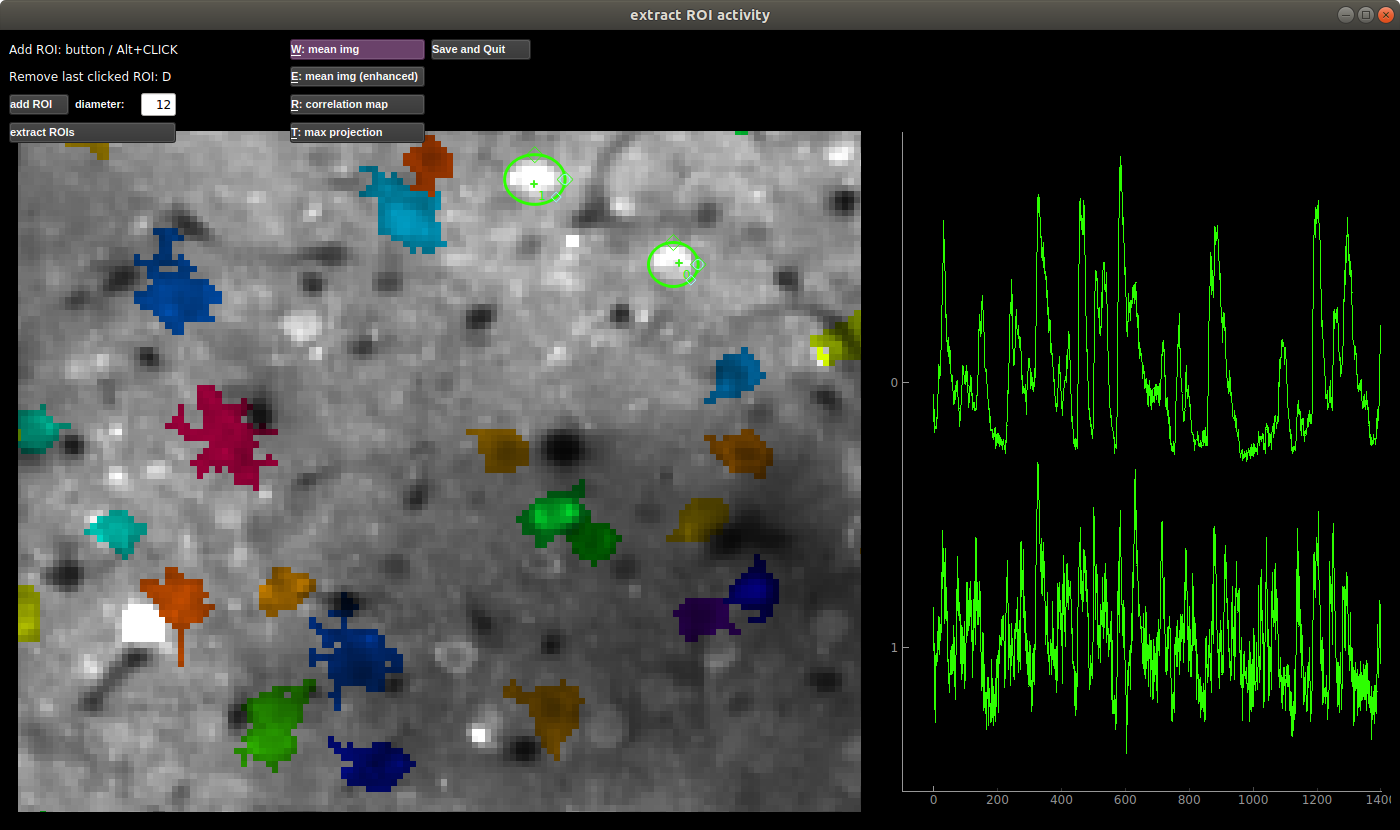
Manual adding of ROIs

You can add ROIs in the File>Manual labelling. You MUST keep the binary file for the computing of the mask’s activity across time. When you save and exit the ROIs will be added to the *.npy files as the first N ROIs (where N is the number that you drew).

Merging ROIs

You can merge selected ROIs (multi-select with CTRL) by pressing ALT+ENTER, or get suggested merges in the “Merge ROI” menu. The merged ROIs then must be saved before you close the GUI to write the new ROIs to the *.npy files. Each merged ROI is appended to the end of the list of ROIs (in stat), and the ROIs that were merged to create it are in the key ‘imerge’. Note in the stat file and other files the original ROIs (that create the ROI) are NOT removed so that you retain the original signals and original suite2p output. In the GUI ROI view the merged ROIs are shown.

The merging of fluorescence is done by taking the mean of the selected cells’ fluorescences. The list of merges are available in the stat for you to choose alternative strategies for combining signals.

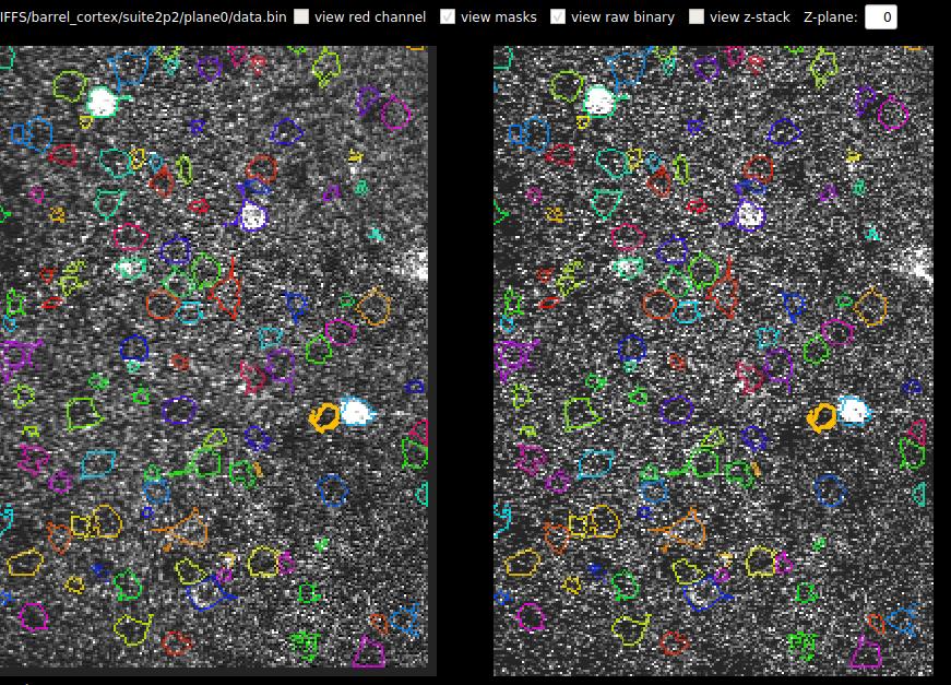
View registered binary

Open the “Registration” menu and click “View registered binary”. A window will pop up with the binary file loaded (first row) along with the registration shifts (second row), and the fluorescence of a selected ROI (third row). If ops[‘keep_movie_raw’]=1, then both the unregistered and registered binaries will be shown in the first row. You can select an ROI by typing in the ROI number in the upper right.

You can zoom in and out on any of the plots. The shift plot and the fluorescence plot have linked x-axes. To return to full view, double-click on the plot that you want to recenter.

When not playing the movie, you can click on the shift plot and the fluorescence plot to go to a specific point in time in the movie. You can also seek through the movie by clicking the slide bar. The left and right arrow keys will move the slide bar incrementally. The space bar will pause and play the movie.

You can also view all the masks, and go from cell to cell by clicking on them.

Z-stack Alignment

You can also now load a Z-stack into this view. You can compute the z-position of the recording across time IF you keep the registered binary file. It expects the Z-stack to be a tiff with number of planes by number of pixels in Y by number of pixels in X. The results of the correlation between z-stack and each frame are saved in ops[‘zcorr’] which is number of planes (in Z) x number of frames. The GUI smooths this matrix across Z and then takes the max and plots the max across time in the third row.

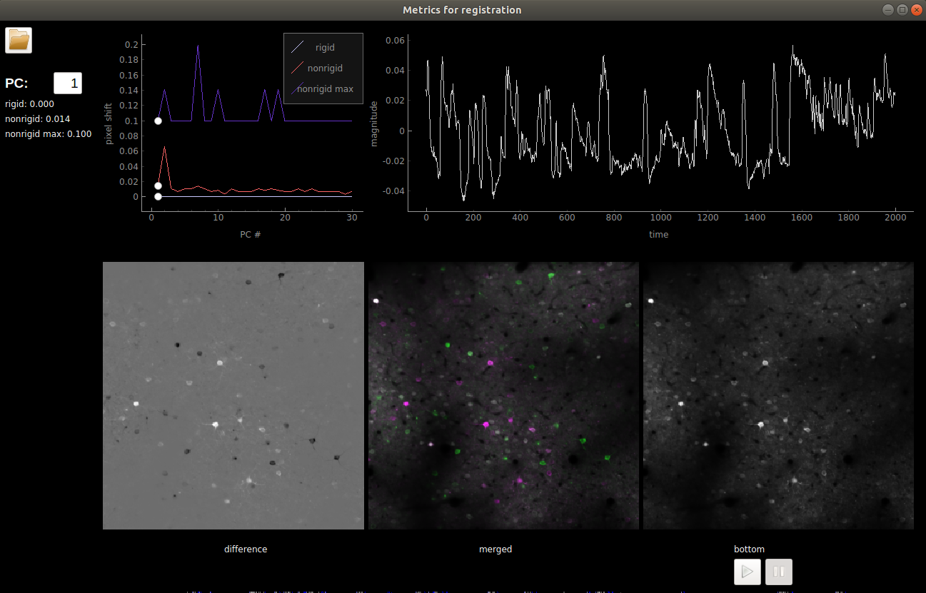
View registration metrics

Open the “Registration” menu and click “View registration metrics”. A window will pop up with ops[‘regDX’] and ops[‘regPC’] plotted. The ops[‘regPC’]’s are computed by taking the principal components of the registered movie. ops['regPC'][0,0,:,:] is the average of the top 500 frames of the 1st PC, ops['regPC'][1,0,:,:] is the average of the bottom 500 frames of the 1st PC. ops['regDX'] quantifies the movement in each PC (iPC) by registering ops['regPC'][0,iPC,:,:] and ops['regPC'][1,iPC,:,:] to the reference images and computing the registration shifts.

The first plot in the upper left shows the magnitude of the shifts (both rigid and non-rigid) in the PCs (ops['regDX']). The second row of plots are meant to help explore the direction of the PC. The first image is the “difference” between the top and the bottom of the PC. The second image is the “merged” image of the top and bottom of the PC. The third image allows you to flip between the top and bottom PCs using the “play” button.

The left and right arrow keys will change the PC number (or you can type in a number). The space bar will pause and play the movie.

The example below shows a movie that has been rigid registered but not non-rigid registered. The metrics suggest that non-rigid registration should also be performed on this recording.